Solution on a regular grid

We shall look in to the solution of (67) on a regular spatial grid, with spacing \(\Delta x\), where the variables \(\eta\) and \(u\) are defined on the same locations:

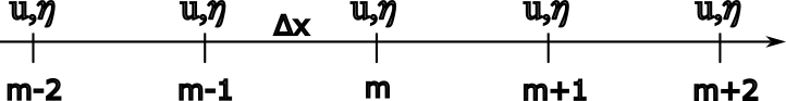
Fig. 11 Regular grid configuration with variables \(u\) and \(\eta\) collocated on the same grid nodes.

Using centred second order differences to discretize the equations for \(\eta\) and \(u\), we obtain the Leapfrog scheme:

(68)\[\begin{align} \frac{\eta_m^{n+1} - \eta_m^{n-1}}{2\Delta t} = -H \frac{u_{m+1}^{n} - u_{m-1}^{n}}{2\Delta x}\\ \frac{u_m^{n+1} - u_m^{n-1}}{2\Delta t} = -g \frac{\eta_{m+1}^{n} - \eta_{m-1}^{n}}{2\Delta x} \end{align}\]

To obtain the discretized version of (67), we take the difference equations defined above and apply centred second-order time and space finite difference formulas, respectively to obtain:

(69)\[ \eta_m^{n+2} - 2\eta_{m}^{n} + \eta_m^{n-2} = gH\frac{\Delta t^2}{\Delta x^2} (\eta_{m+2}^{n} -2\eta_{m}^{n} + \eta_{m-2}^{n}) \]

The discretization we obtain is based on grid points and time steps that are \(2\Delta x\) and \(2\Delta t\) apart, which implies a truncation error of magnitude \(O(4\Delta x^2, 4\Delta t^2)\), which is larger than the typical \(O(\Delta x^2, \Delta t^2)\) magnitude of the Leapfrog scheme truncation error.

Another issue with the regular grid approach is the \(2\Delta x\) spacing that appears in (69). This effectively decouples the even and odd grid positions, as the computations on the even grid nodes do not “see” the data of the odd grid nodes (see Figure Fig. 12).

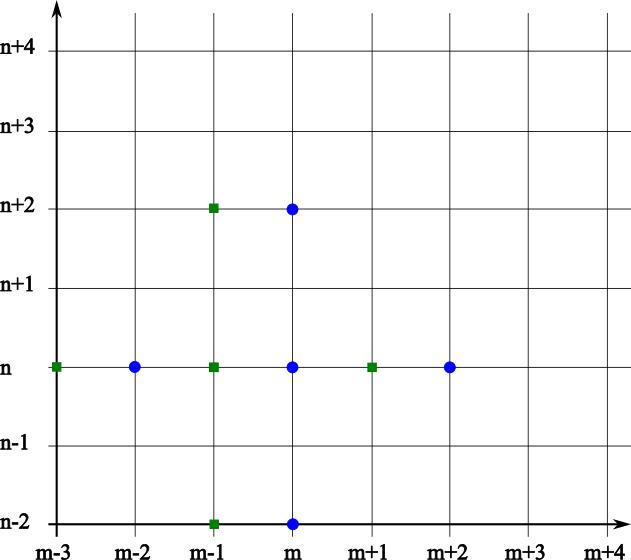
Fig. 12 Decoupling of even (blue circles) and odd (green squares) in the decourse of the computations.

This will lead to unacceptable solutions, such as stationary \(\eta\) that alternates between constant positive and negative values. Stationary solutions are related to the null space of the spatial derivative operator \(\mathcal{S}\) of (69):

(70)\[ \mathcal{S}(\cdot) = gH [(\cdot)_{m+2}^{n} -2(\cdot)_{m}^{n} + (\cdot)_{m-2}^{n}]. \]

The members of the null space of \(\mathcal{S}\) are the solutions of \(\mathcal{S}(x)=0\). For a solution \(\eta(m\Delta x,t) = \eta_0 e^{\imath(km2\Delta x - \omega t)}\), the null space is the solution of:

(71)\[ \mathcal{S}(\eta) = gH (e^{\imath2k\Delta x}-2+e^{-\imath2k\Delta x})=-\frac{4gH}{\Delta x^2}\sin^2\left( \frac{k\Delta x}{2} \right)\cos^2\left( \frac{k\Delta x}{2} \right)=0 \]

which is true for the \(2\Delta x\) wave length, which is the smallest wave length that can be resolved in a grid of spacing \(\Delta x\).

The expression for the null space of (69) can also be used to derive the dispersion relation implied by the Leapfrog scheme. To obtain this, we cast (67) in a semi-discretized form:

\[ \frac{\partial^2 \eta}{\partial t^2} + \mathcal{S}(\eta) = 0 \]

that, upon substitution of the wave form solution becomes:

\[ \omega^2 = \frac{4gH}{\Delta x^2}\sin^2\left( \frac{k\Delta x}{2} \right)\cos^2\left( \frac{k\Delta x}{2} \right). \]

which is significantly different from the analytic dispersion relation \(\omega^2 = gHk^2\).